14 Understanding Time Series Data
14.1 What is Time Series Data?
This chapter introduces the concept of time series data and its analysis. Time series analysis (TSA) is the study of data points collected or recorded in time order. Such data are called time series data.
Unlike other types of observations, time series data allows us to examine patterns over time, such as trends, seasonality, or random fluctuations. This is because we can make certain assumptions about such data, based on the fact that it has been collected in time order.
Usually, time series analysis is used to understand historical behaviour, identify meaningful patterns, and predict future values. Underpinning these goals, the principle objective of time series analysis is to understand the structure of the data.
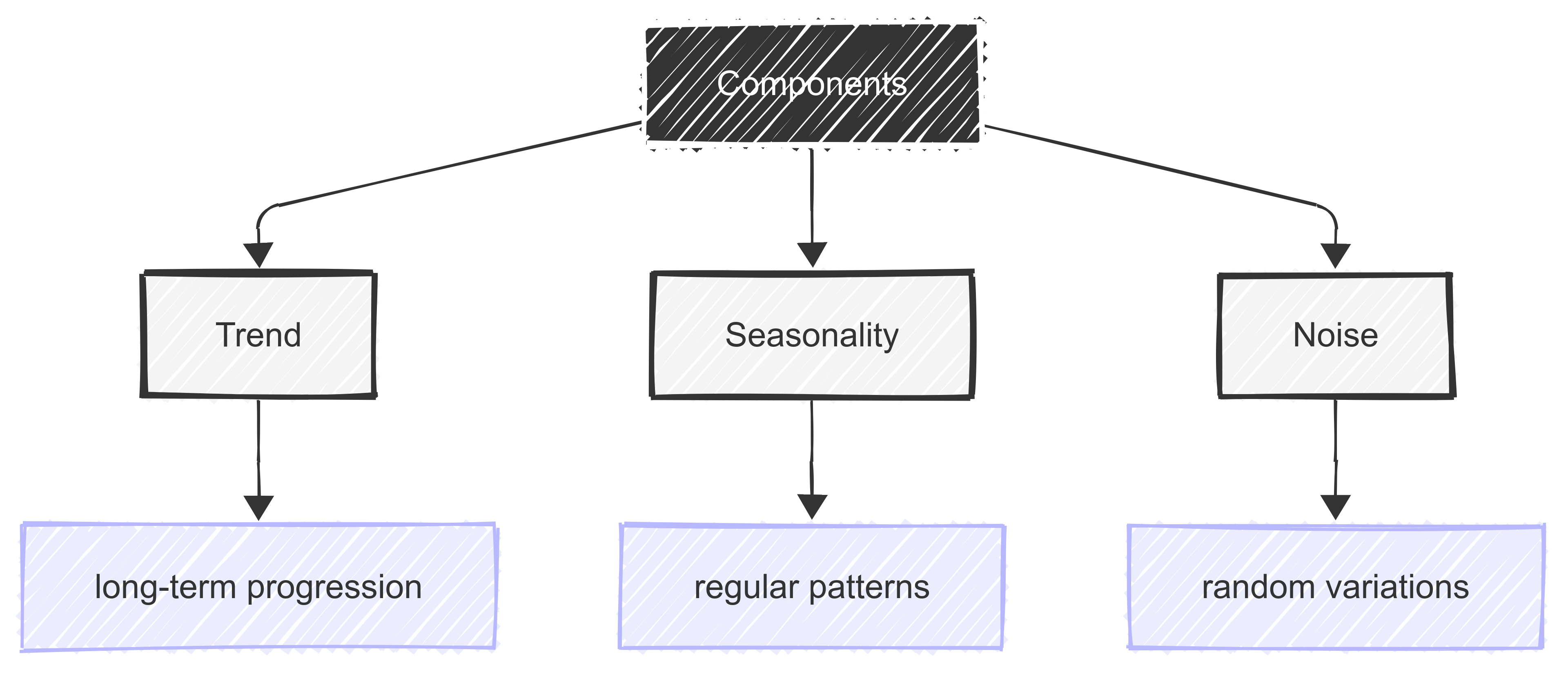
There are three key elements to this structure:
the trend - the long-term direction of the data;
seasonality - regular, repeating patterns in the data (e.g., shop sales peaking every December); and
noise - random variations in the data with no clear pattern.
The goal of TSA is to model these three components to help make better decisions or forecasts about the future.
14.2 Characteristics of Time Series Data
14.2.1 Introduction
Before we explore the analysis of time series data, it’s important to understand its characteristics.
Note
Time series data consists of observations collected sequentially over time, making it fundamentally different from standard cross-sectional data.
Unlike independent data points, time series observations are often autocorrelated. This means that past values influence future values.
The temperature today is influenced by the temperature yesterday, so it’s not independent.
Key characteristics of time series data include trend, which represents long-term upward or downward movement; seasonality, which describes recurring patterns at fixed intervals (e.g., monthly or yearly cycles); and stationarity, where statistical properties such as mean and variance remain constant over time.
Additionally, time series data often contains random noise unpredictable fluctuations that obscure underlying patterns.
14.2.2 Time-ordered data points
Introduction
We’ll begin by reviewing the essence of time series data: that it contains time-ordered data points.
Time-ordered data points are sequential measurements or observations that are recorded along with their corresponding timestamps. These data points form a time series, and thus allow us to analyse patterns, trends, and changes over time.
Examples
In sport, time-ordered data points we might have to deal with include:
- Match scores and statistics, tracked period by period or minute by minute;
- Player performance metrics like running speed, distance covered, and heart rate during games;
- Team rankings and standings throughout a season; or
- Individual athlete’s personal records and progression over time.
Each of these variables has an element of time-ordering, and therefore requires careful consideration with regard to its analysis.
Key characteristics
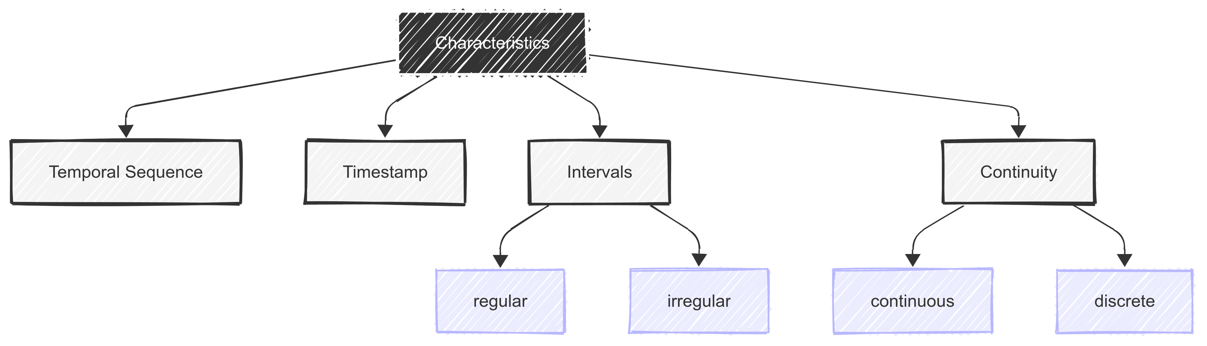
To develop this idea further, it’s important to note that time series data has the following characteristics, which separate it from other types of continuous data:
- A temporal sequence: Data points are arranged chronologically;
- A timestamp association: Each data point has a specific time reference (time, date etc.);
- Regular or irregular intervals: Measurements can be taken at fixed or variable time gaps; and
- Can be continuous or discrete: Data can be continuous (like temperature) or discrete (like daily sales).
Analysis methods
Because of its unique structure, there are a number of useful/interesting things we can do with such data.
For example:
- Trend analysis: We can identify long-term patterns in the data;
- Seasonality detection: We can explore recurring patterns that occur at regular intervals;
- Forecasting: We can predict future values based on past data; and
- Anomaly detection: We can identifying unusual patterns or outliers in the data.
We’ll cover each of these approaches later in the chapter.
14.2.3 Single vs. multiple variables
It’s important to note that time series data can involve either a single variable (univariate time series) or multiple variables (multivariate time series).
A univariate time series consists of observations for one variable recorded sequentially over time, such as daily weight measurements, or weekly points totals.
In contrast, a multivariate time series tracks multiple related variables over time, such as heart rate, temperature, and velocity recorded simultaneously.
Multivariate time series analysis allows for significant insights by capturing interactions between variables, often leading to improved forecasting accuracy. However, it also introduces greater complexity, requiring the use of specialised models that account for dependencies between multiple time-dependent variables.
14.2.4 Regular or irregular intervals
Time series data can also be recorded at regular or irregular intervals.
Regularly spaced time series have observations collected at consistent time steps, such as daily, monthly, or yearly measurements. This structure simplifies analysis and enables the use of standard statistical models.
Irregular time series, on the other hand, involve observations recorded at uneven intervals, such as financial transactions occurring at random times or medical events logged based on patient activity.
Analysing irregular time series often requires interpolation, resampling, or specialised models that can handle unevenly spaced data while preserving temporal relationships. Recognising the nature of time intervals in our data is crucial for selecting appropriate analytical techniques.
14.3 Components of Time Series Data
As noted above, the structure of time series data can be broken down into three fundamental components that help us understand and analyse patterns in such data.
We’ll explore each of these components in more detail below.
14.3.1 Trend
Introduction
A trend in time series data represents the underlying pattern or direction that emerges when observing data points over an extended period.
It reflects the general movement of a variable through time, abstracting away from short-term fluctuations and seasonal variations. Trends can be upward (increasing), downward (decreasing), or horizontal (stable), providing important insights into the long-term behaviour of the data.
Types of trend
Understanding trends can help us identify persistent patterns that may continue into the future.
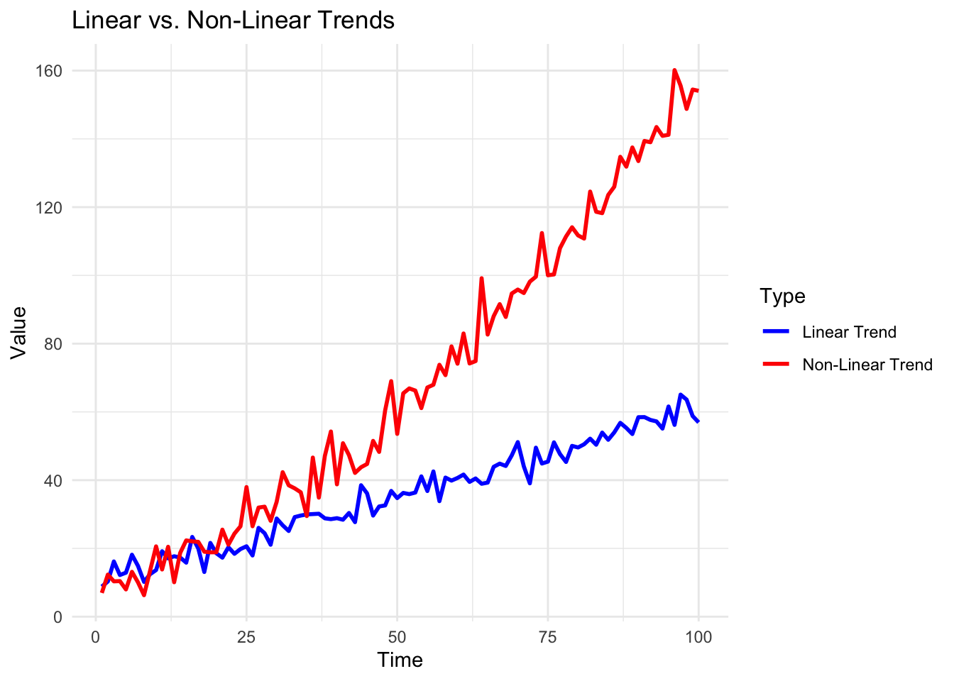
For example, trends can be linear, showing a consistent rate of change, or nonlinear, displaying varying rates of change over time.
The process of trend analysis often involves sophisticated statistical techniques to separate the trend component from other elements like seasonal patterns, cyclical fluctuations, and random variations. We’ll cover this shortly.
Why is trend analysis useful?
In practical applications, trend analysis serves multiple purposes. It aids in forecasting future values, because we usually assume that the trend will continue. It therefore supports decision-making, and helps identify significant changes in the underlying phenomenon we are studying.
How are trends measured?
The ability to accurately identify and analyse trends is important for making informed predictions and understanding the fundamental direction of time-dependent processes.
A number of methods exist for identifying and measuring trends, ranging from simple visual inspection to complex mathematical models.
Common techniques include:
moving averages;
regression analysis; and
exponential smoothing.
These methods help in smoothing out short-term fluctuations and highlighting the underlying trend, making it easier to understand the data’s long-term behaviour and make more accurate predictions about future developments.
14.3.2 Seasonality
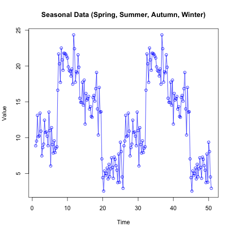
Seasonality refers to recurring patterns within a time series that follow a regular interval, such as every month or every quarter.
In many real-world contexts, like retail sales, tourism, or passenger numbers, these fluctuations may be tied to the calendar, holidays, or climate. Detecting seasonality helps us understand and anticipate recurring cycles, enabling more accurate forecasting and resource allocation.
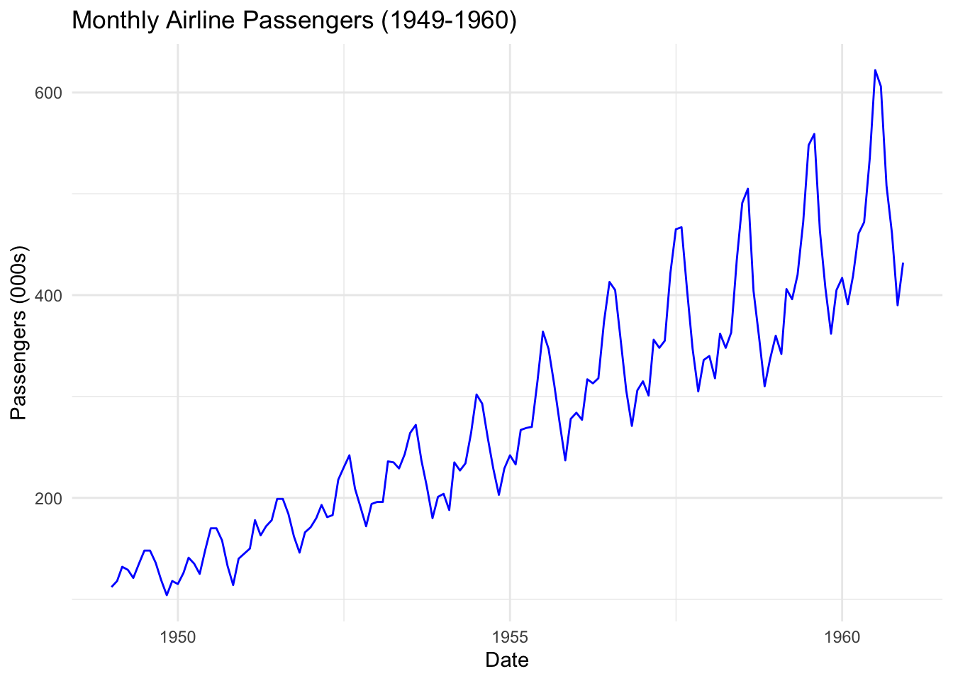
In the AirPassengers dataset (included in R), for instance, peaks typically appear in mid-year, reflecting increased travel during summer months in the Northern Hemisphere.
Accounting for this cyclical movement is essential for interpreting underlying trends and making precise predictions. Ignoring seasonality can obscure the true nature of the data and lead to suboptimal decisions.
14.3.3 Noise
Noise in a time series refers to the random, unpredictable variation that is not explained by trends, seasonality, or other systematic components. It’s like static in a radio signal; always present, but not necessarily informative about the underlying process. In practice, noise can arise from measurement error, short-term fluctuations, or small random shocks.
Recognising the level of noise in a time series is crucial for building reliable models. If noise dominates, any effort to identify meaningful patterns or trends becomes more challenging.
Statistical methods often attempt to filter out noise, leaving the more predictable components of the data. By understanding how much variation is random versus systematic, we can set realistic expectations for forecasting accuracy.
14.4 Visualising Time Series Data
14.4.1 Introduction
Because of its nature, time series data benefits from visualisation. Visualisation is an important step in time series analysis, helping us understand trends, seasonal patterns, and potential anomalies in our data.
14.4.2 Line plots for trends
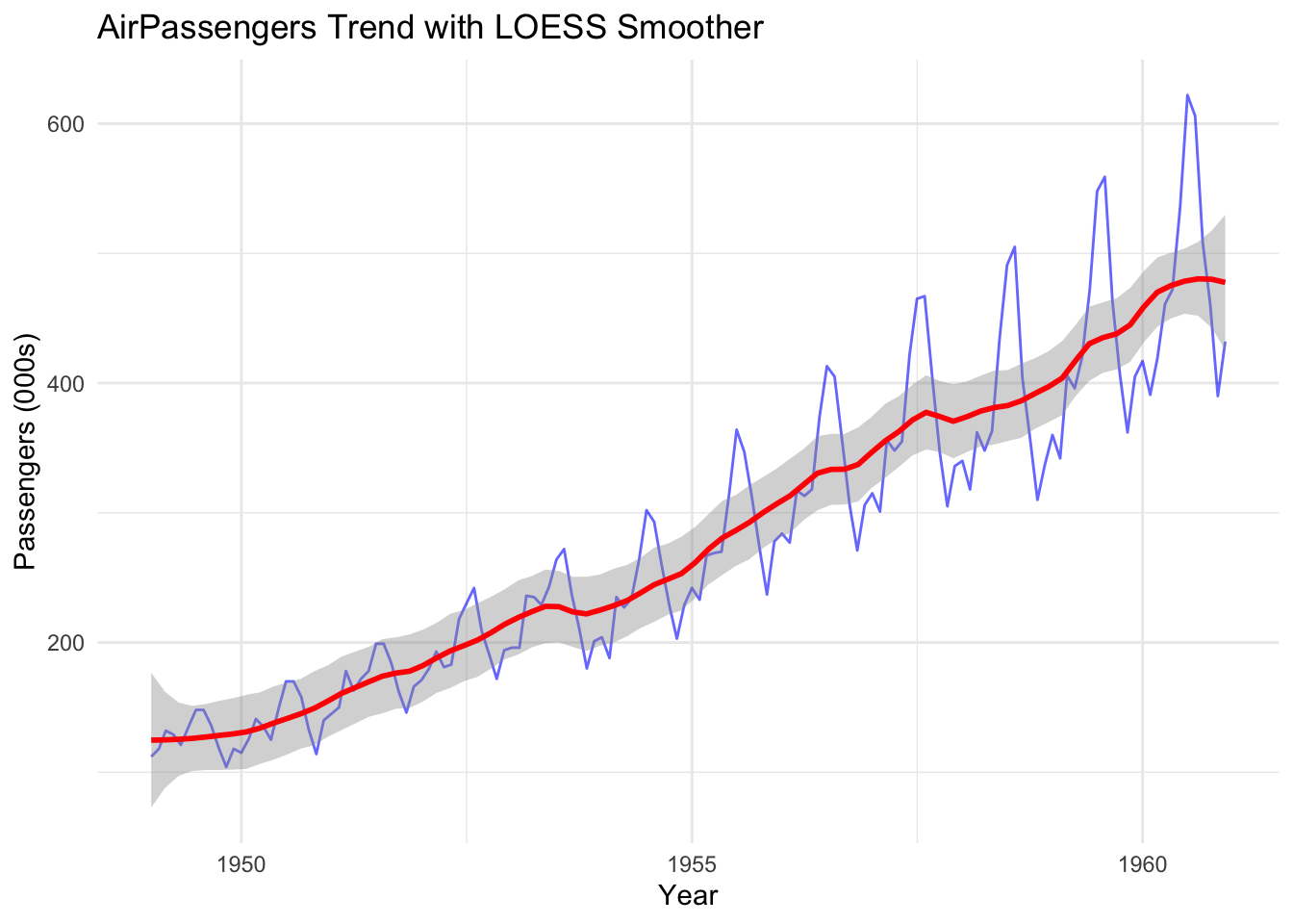
Line plots are often the first choice for displaying time series data over time. They make it easy to spot increasing or decreasing trends, sudden shifts, and any recurring cycles.
By focusing on the long-term direction, line plots help separate systemic behaviour from short-term noise.
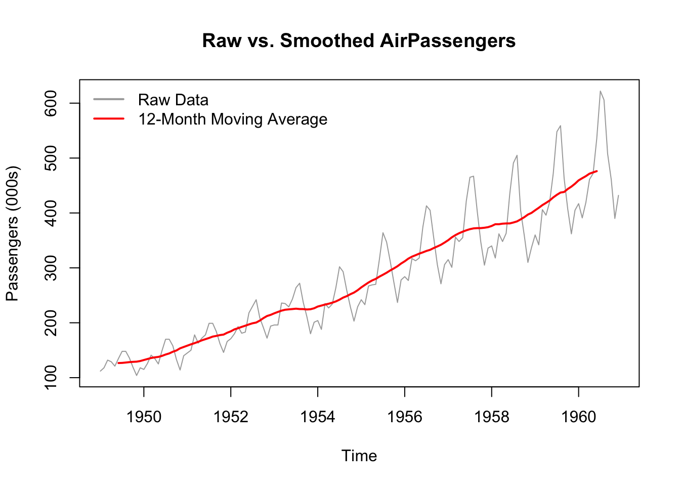
In the following example, the line plot (in red) helps us see the underlying trend in the data that might not be apparent in the original plot. This is a result of applying a smoothing function to the raw data.
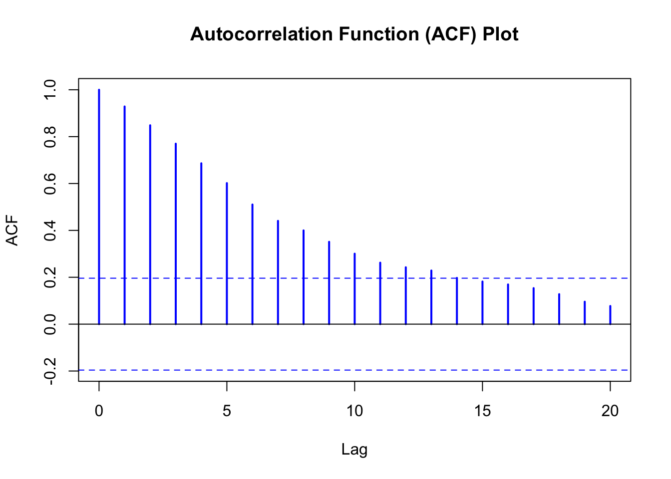
14.4.3 ACF for lag analysis
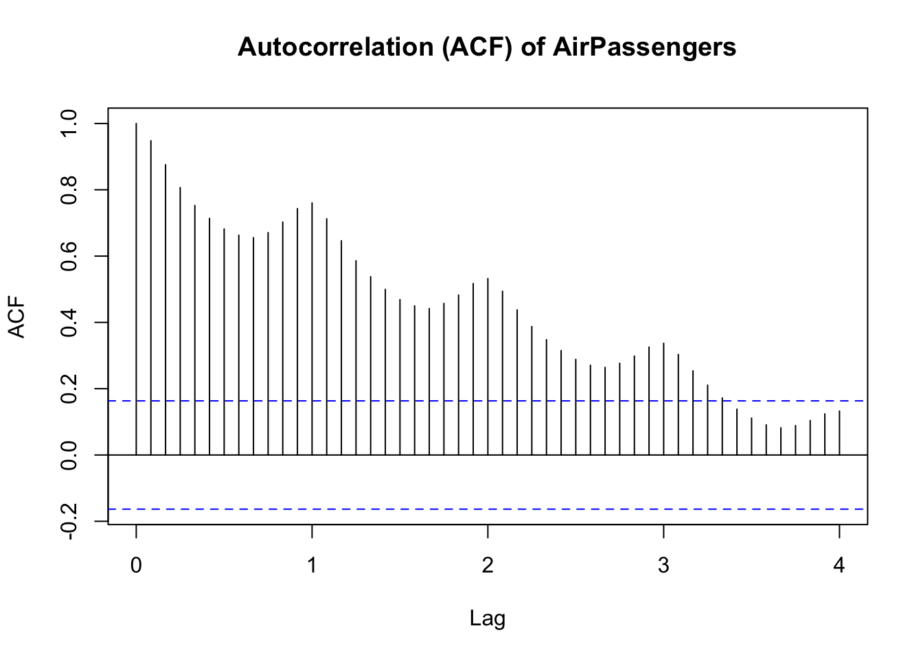
Another type of plot, called an Autocorrelation Function (ACF), shows how a time series is correlated with itself at different lags.
Large positive spikes can signal persistent trends or seasonal effects, while negative spikes might indicate mean-reverting behavior.
The term ‘lag’ refers to the delay between observations when measuring correlation. In a monthly data set, lag 12 would mean looking at the correlation between the current observation and the observation one year ago (12 observations back).
ACF plots are essential for diagnosing the underlying data-generating process, guiding the selection of analytical models like ARIMA that we’ll cover later in the module.
14.4.4 Seasonal breakdowns
Seasonal breakdowns help us see how each season (or month, quarter, etc.) behaves year by year.
This is done by decomposing the series, separating it into trend, seasonal, and residual (noise) components. These breakdowns are invaluable for forecasting and clarifying the distinct parts of variation within the series.
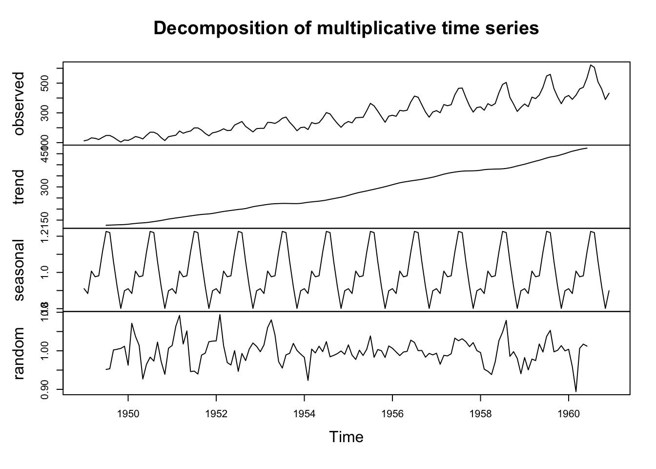
Notice that the figure is composed of four elements:
Observed Series (Top Panel)
This displays the original time series data.
This gives a first impression of overall trends, seasonality, and variability.
Trend Component (Second Panel)
This shows the long-term progression of the data, smoothing short-term fluctuations.
If the trend is increasing or decreasing, it suggests a systematic change over time.
A flat trend indicates no significant long-term movement.
Seasonal Component (Third Panel)
This panel captures repeating patterns within a fixed period (e.g., monthly or yearly cycles).
If peaks and troughs occur consistently at the same time intervals, strong seasonality is present.
For example, in retail sales data, an increase every December would suggest a holiday shopping effect.
Residual (Random) Component (Bottom Panel)
This represents unexplained variation after removing trend and seasonality.
Ideally, residuals should be randomly distributed around zero.
Large residual fluctuations suggest the presence of additional irregular influences or missing structural components.
14.5 Autocorrelation in Time Series Data
14.5.1 Introduction
Autocorrelation is a significant feature of time series data, and (IMO) is often ignored in sport data. It measures how a time series correlates with its own past values.
High autocorrelation suggests that past observations heavily influence the current state, which can be vital for forecasting and understanding the momentum or inertia in a series.
Low or no autocorrelation implies that past values provide limited information about future outcomes.
In the following ACF plot, we can see the correlation coefficient (y-axis) between each point and its lag (how many time steps back we compare) on the x-axis. The figure suggests that each observation has a correlation of around 0.6 with the observation 5 time steps ago (‘time step’ could be a minute, an hour, a day etc.)
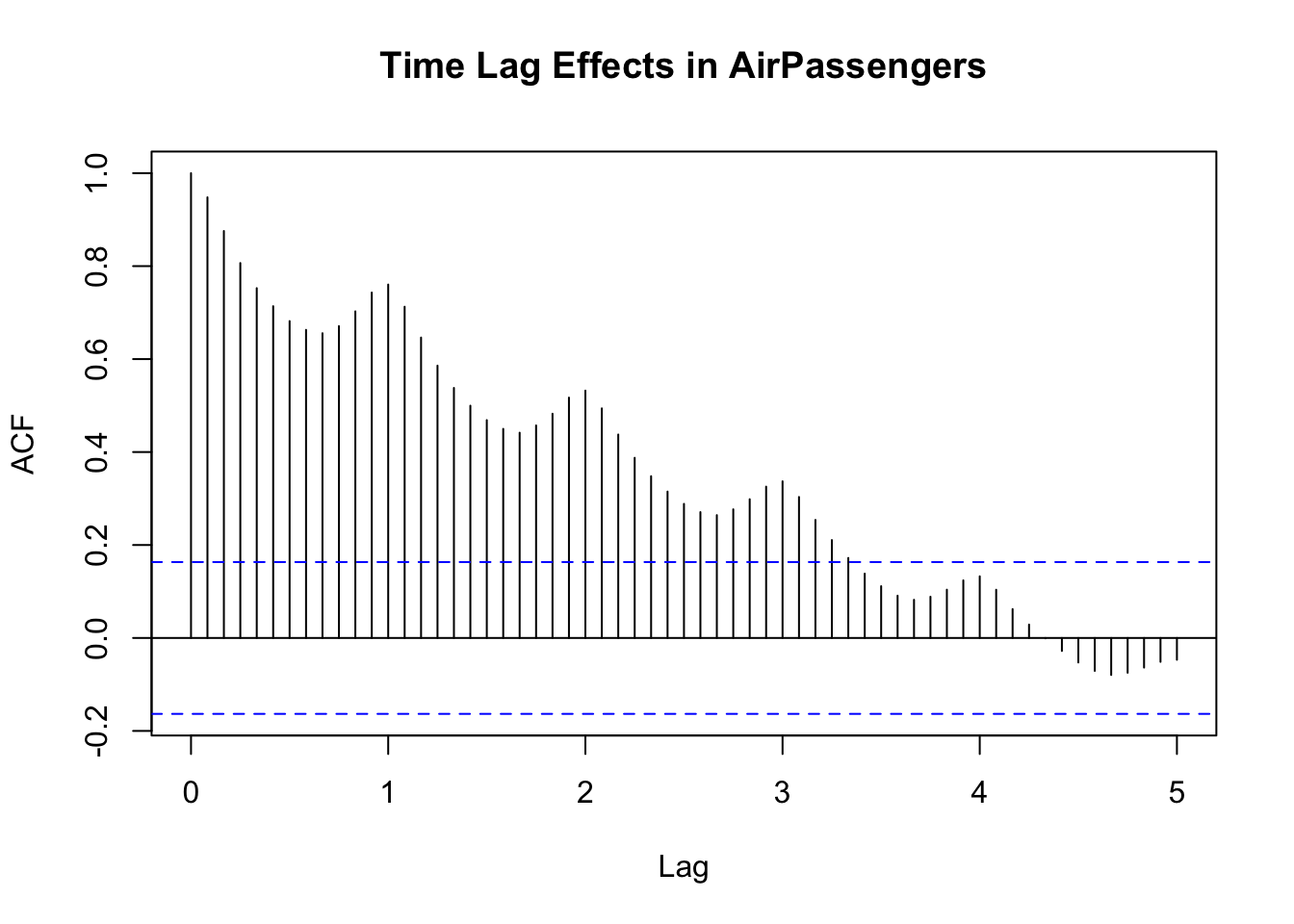
14.5.2 Time lag effects
Time lag effects are the specific delays after which correlations appear. For instance, in monthly data, a strong correlation at lag 12 might reflect yearly seasonality. Recognising these lags helps determine if the current data point depends on observations from one month ago, one year ago, or both, guiding model selection.
Notice in the following figure (where the values in the x-axis represent years) that there is a clear element of seasonality in the correlations.
14.5.3 Positive and negative correlation
When an autocorrelation spike is positive, it indicates that if the series was above average in a given period, it tends to remain above average after that specific lag.
Negative autocorrelations mean that if the series is high in one period, it’s likely to be low after the specified lag, hinting at oscillatory or mean-reverting tendencies.
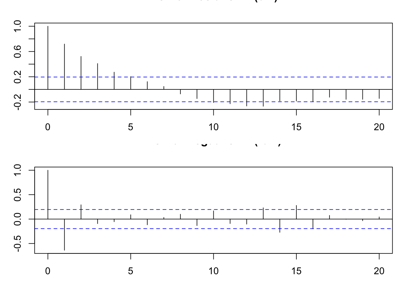
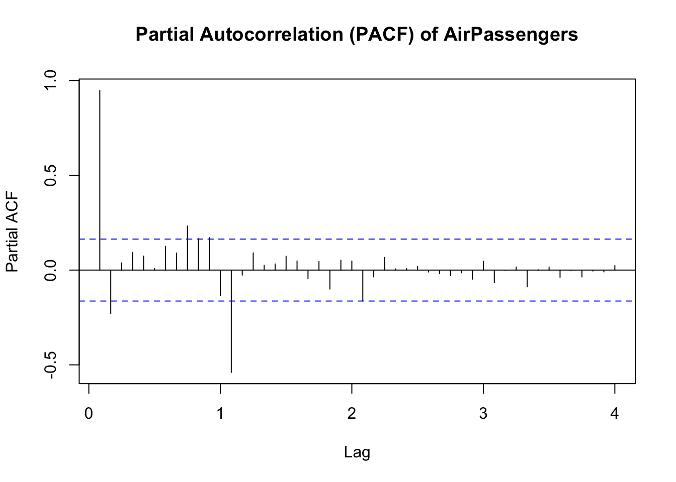
14.5.4 PACF analysis
A Partial Autocorrelation Function (PACF) helps distinguish direct correlations from those explained by intermediary lags.
For instance, a significant spike at lag 1 in the PACF suggests that past observations one period back have a direct influence on the current value.
By contrast, if the ACF at lag 2 is large but the PACF at lag 2 is small, it implies that the lag-2 effect is mostly due to lag-1 dependence.
14.6 Conclusion
In this chapter, we’ve covered some basic ideas about time series data, its characteristics, and how we might begin to understand its structure through visualisation.